Aggregation and Window

In this tutorial you will learn how to write aggregation queries and learn about the window concept in Odysseus.

We will use the same setting as in Simple Query Processing. So you should follow steps 1-4.

Aggregation

Odysseus provides a wide range of aggregation operators. In this tutorial we will focus on the typical aggreations average (AVG), count (COUNT), sum (SUM), minimum (MIN) and maximum (MAX).

Crate a new Odysseus Script file with the PQL template an name it aggregation1. Change #RUNQUERY to #ADDQUERY. By this, the query will only be installed an not started, so its easier to see what happens.

Write the following query:

#PARSER PQL
#TRANSCFG Standard
#ADDQUERY
out = AGGREGATE({
          aggregations=[['COUNT', 'price', 'COUNT_price', 'integer']]
        },
        nexmark:bid
      )

Here you can see the aggreation operator that connects to source nexmark:bid. The aggregate functions are defined by the aggregations parameter. In this example you can see four entries. The first entry defines the aggreagte function, COUNT in this case. The second entry, the attribute can should be used for the aggregation. For COUNT is does not matter, which attribute of the input element should be treated, but one attribute must be given, so be choose price. The third parameter defines the name of the output attribute, i.e. what is the new name for the output and finally, the last parameter determines the output data type. This parameter is optional.

Now execute the script, and show the result stream (e.g. as a table). Now start the query (e.g. with the selection of the Start Query Button).

The result should be something like this:

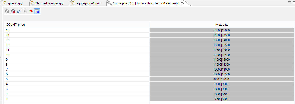
Here you can see 15 bids that have entered the system.

Other aggregations can be added easily, by adding another value to the aggregations parameter.

Remove the old query.

In the Project Exploer

right click on the aggregation1.qry file and choose Copy
right clock on the Project Name (FirstSteps) and choose Paste
Enter a new name for the query: aggregation2.qry
Open the new file by double clicking in the project explorer

Replace the input with the following:

#PARSER PQL
#TRANSCFG Standard
#ADDQUERY
out = AGGREGATE({
          aggregations=[
            ['COUNT', 'price', 'COUNT_price', 'integer'],
            ['AVG', 'price', 'AVG_price'],
            ['SUM', 'price', 'SUM_price'],
            ['MIN', 'price', 'MIN_price'],
            ['MAX', 'price', 'MAX_price']
          ]                
        },
        nexmark:bid
      )

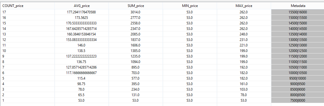
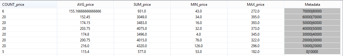
The results of the query should look somehow like the following:

Now its time to highlight the Metadata part a little more.

In the last column you can see two values, separated by "|". The two values show the validity of the event. 7500|8000 e.g. means, that this event was valid in real time starting at 7500 (in Nexmark this means after 7.5 seconds) and ends before 8000, mathematical this is a right open interval: [7500,8000).

If you look at the values, you can see that they are not overlapping. This should be rather clear, because the count e.g. can not be 1 and 2 at the same time. The metadata show, that every 500 (in this case milliseconds) a new bid is send to the system and a new aggregation is build.

Another important think to note is, that a new aggregation will be calculated, when a new event arrives a the system. For this example it take 8 seconds before the first value is created. For streams with a low data rate the AssureHeartbeat operator can be used to produce values on a regular base.

There is also the possibility to define groups (as in SQL group by). The below in Element Based Windows for an example.

Window

In the example above you can see that the aggregated values always contain the information of all previous events.Typically, the older the event is, the less interesting is it. An auction system provider may not only be interested in the alltime highest bit, but e.g. the highest bit for a specific time (e.g. the last 24 hours) or related to a number of bit that have been posed.

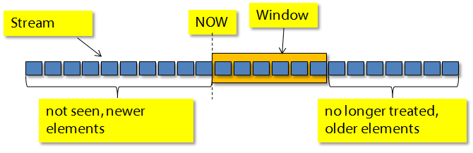
For this, Odysseus allows to define windows. A window defines a subset of elements that should be treated together, e.g. should be aggregated.These subset can overlap (so called sliding windows) or be disjunct (tumbling windows).

The following picture shows such a window. In this case 6 elements are in the window.

Odysseus provides three types of windows:

Time based
Element based
Predicate based

Time Based Window

The time based window allows to define windows based on the time.

Create a new PQL script and name it timewindow1:

#PARSER PQL
#TRANSCFG Standard
#ADDQUERY
out = TIMEWINDOW({SIZE=10000},nexmark:bid)

In this example we define a time based window over the bid source with a size of 10000, here 10 seconds.

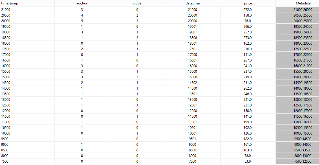
If you run the query and look at the results you will see something like this:

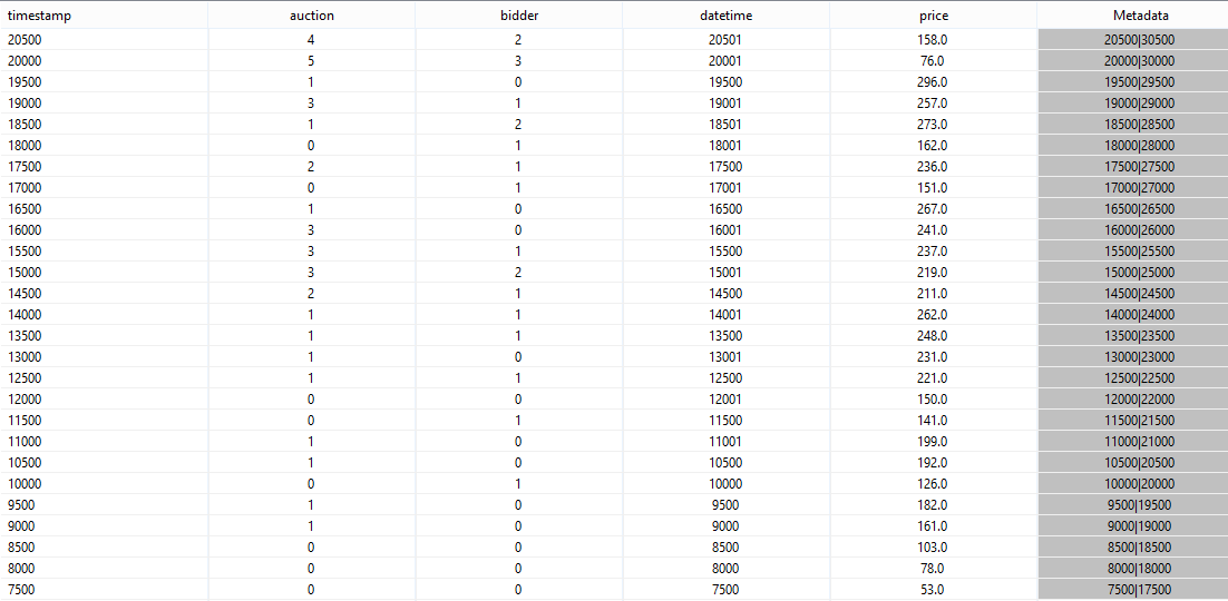
If you look at the metadata you can see that each element has a time interval ranging from it start timestamp to a future time that lies 10000 ahead, e.g. 7500 to 17500, 8000 to 18000 and so on. The meaning of the time is, that elements that are valid at the same time should be treated together. If you look e.g. at time 10000 there are 6 events which time interval contains this value. The seventh element (with start time stamp 10500) is part of another window.

We can now combine the window with the aggregation.

Remove the running query.

Create a new PQL query (window_aggregation1) with the following input:

#PARSER PQL
#TRANSCFG Standard
#ADDQUERY
windowed = TIMEWINDOW({SIZE=10000},nexmark:bid)
out = AGGREGATE({
          aggregations=[
            ['COUNT', 'price', 'COUNT_price', 'integer'],
            ['AVG', 'price', 'AVG_price'],
            ['SUM', 'price', 'SUM_price'],
            ['MIN', 'price', 'MIN_price'],
            ['MAX', 'price', 'MAX_price']
          ]                
        },
        windowed
      )

If you run the query the result should look like this:

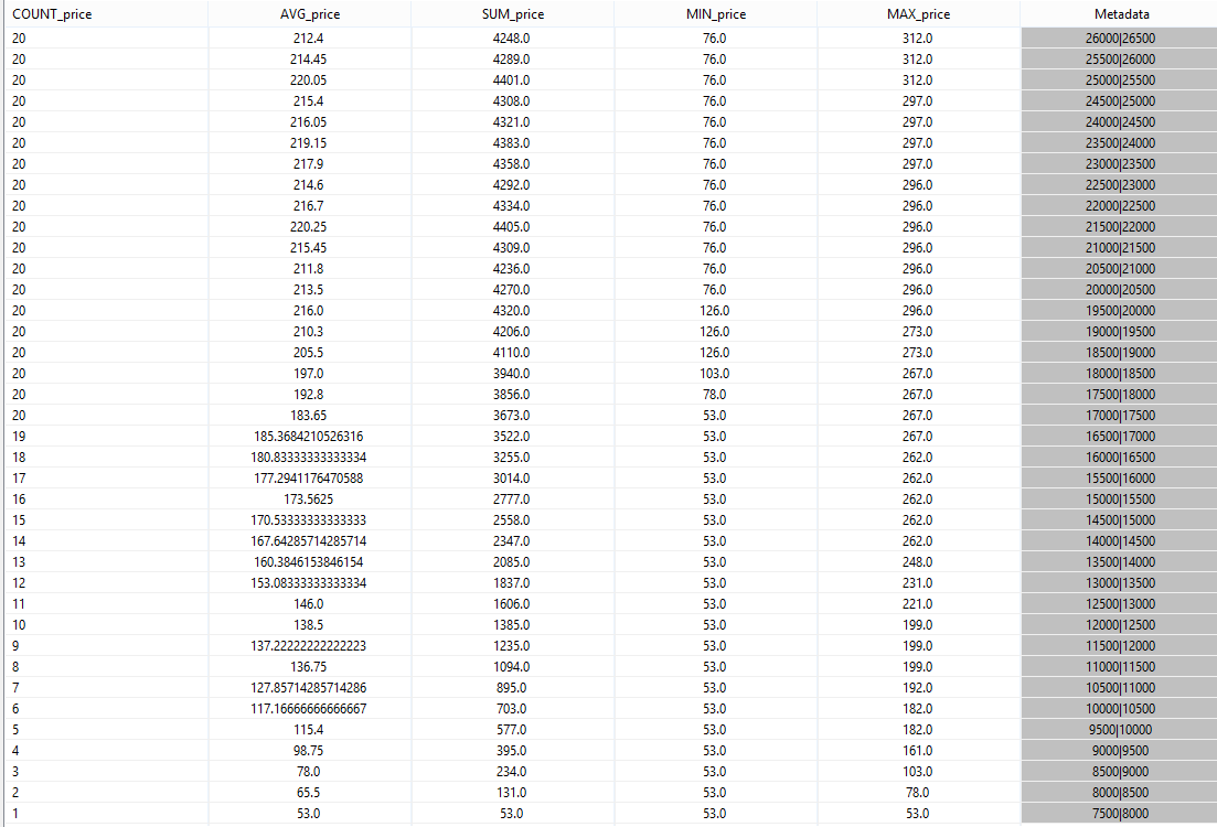
You can see, that the count attribute is counted up to 20. This mean that in this case 10000 (here 10 seconds) contains 20 events. If you look at the result of the above window query, you can see that the first and the twentieth element have an overlapping time stamp, and the 21th element not. So the new window only treats element 2 to 21.

Note, in this szenario the elements are generated in a constant fashion, so the size of the window is always 20. In "real" szenarios this is typically not the case and the size of the windows in terms of containg elements differ (e.g. count the number of cars for an hour).

The window we defined is called a sliding window. The query delivers the aggregations about the bids that were posed in the last 10 seconds.

Sometimes, the result should not be in a sliding way. E.g. if a provider wants to know how many bids are posed in 10 second intervals. If the size is 10 seconds, this is called a tumbling window.

A tumbling window can be defined with one of the two parameters: ADVANCE or SLIDE. The difference is how the start time stamp of the elements in the window are treated. Let us start with ADVANCE.

Remove all running queries.

Create a new PQL script timewindow2.qry as in the following:

#PARSER PQL
#TRANSCFG Standard
#ADDQUERY
out = TIMEWINDOW({SIZE=10000, ADVANCE=10000},nexmark:bid)

Running should show you something like this:

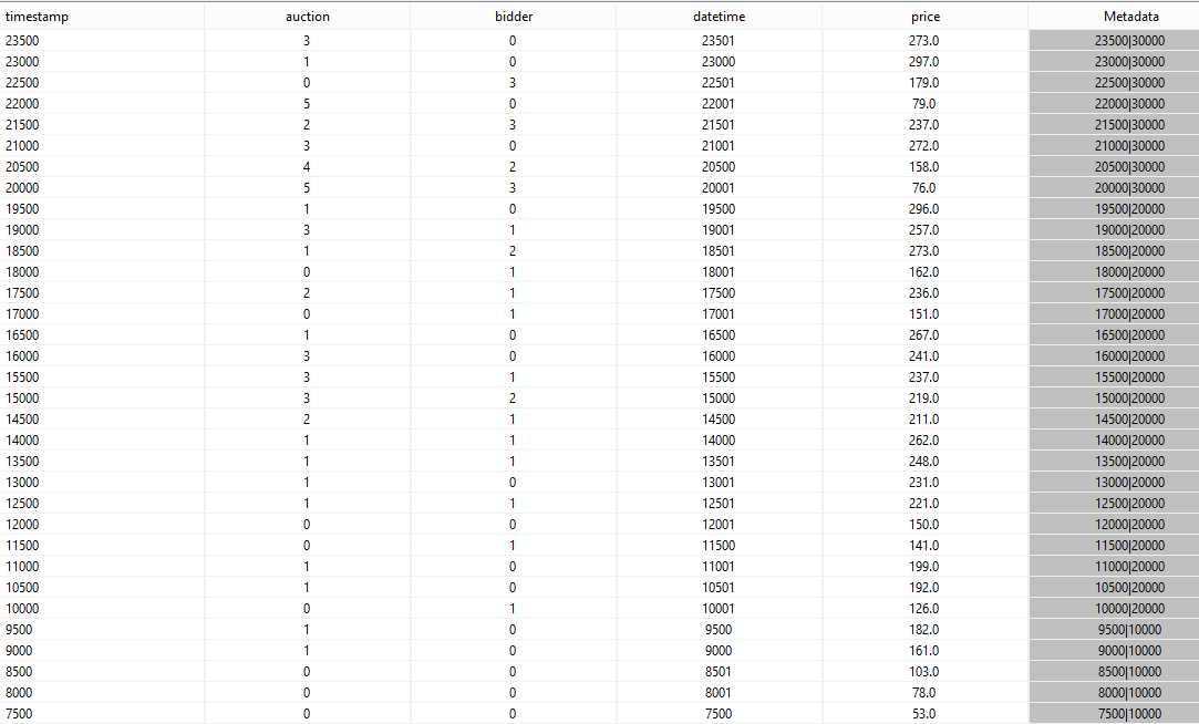
You can see, that the timestamps are different. Each events belonging to the same window has the same end time stamp (e.g. 10.000, 20.000, 30.000).

If you run the following aggregation query (window_aggregation2)

#PARSER PQL
#TRANSCFG Standard
#ADDQUERY
windowed = TIMEWINDOW({SIZE=10000, ADVANCE=10000},nexmark:bid)
out = AGGREGATE({
          aggregations=[
            ['COUNT', 'price', 'COUNT_price', 'integer'],
            ['AVG', 'price', 'AVG_price'],
            ['SUM', 'price', 'SUM_price'],
            ['MIN', 'price', 'MIN_price'],
            ['MAX', 'price', 'MAX_price']
          ]                
        },
        windowed
      )

you will see the following output (when no other query is running!):

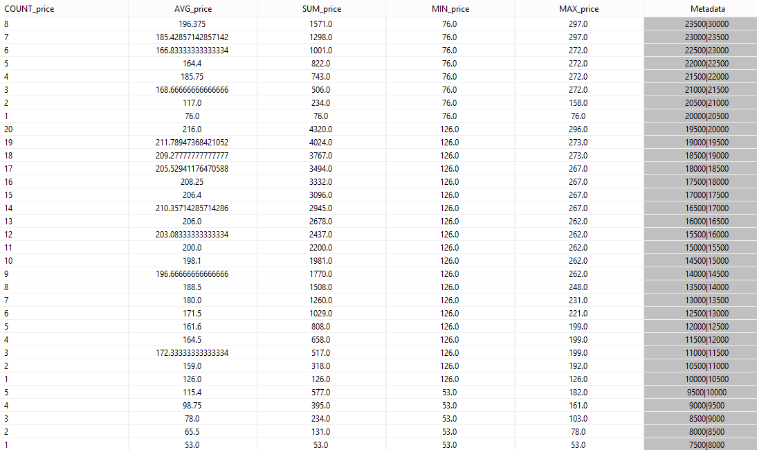
As you can see, the aggregations count up to 20 and then start again at 1. This is not exactly, what the provider wanted. The problem here is, that the elments have different start time stamps and only those parts of the elements are aggregated where the time intervals overlap.

A way to cope with this is to use another parameter called SLIDE. With slide all start timestamp are set to the same value. This can be interpreted as reducing the granularity of the time domain.

So remove all queries. A start a new PQL query (timewindow3)

#PARSER PQL
#TRANSCFG Standard
#ADDQUERY
out = TIMEWINDOW({SIZE=10000, SLIDE=10000},nexmark:bid)

After starting this query, you should see something like:

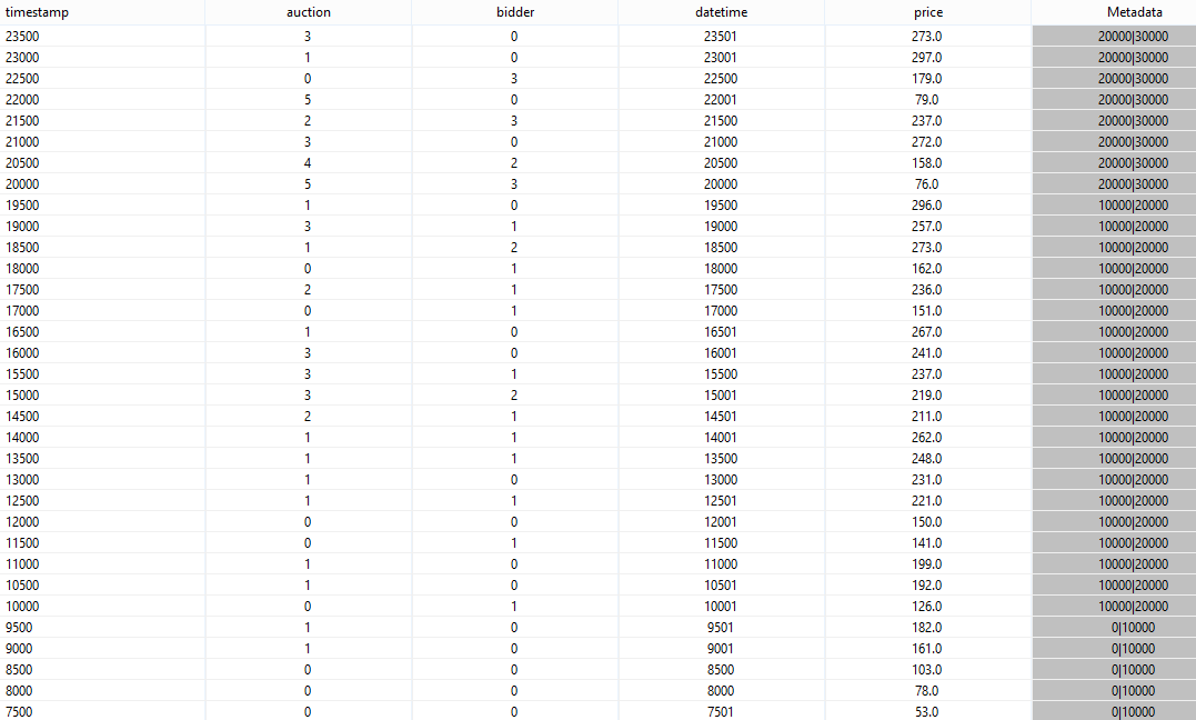
Now you can see, that for one window all time intervals are the same.

If we now run the following query (window_aggregation3):

#PARSER PQL
#TRANSCFG Standard
#ADDQUERY
windowed = TIMEWINDOW({SIZE=10000, SLIDE=10000},nexmark:bid)
out = AGGREGATE({
          aggregations=[
            ['COUNT', 'price', 'COUNT_price', 'integer'],
            ['AVG', 'price', 'AVG_price'],
            ['SUM', 'price', 'SUM_price'],
            ['MIN', 'price', 'MIN_price'],
            ['MAX', 'price', 'MAX_price']
          ]                
        },
        windowed
      )

You will get the following output:

Note: You could ignore the first line, it was created because when the query was stopped.

Here you can see the aggregation over 10 second intervals.

Element Based Window

Another way to define a window, is based on elements, e.g. the last 10 elements received. In Odysseus, the element based window is implemented with timestamps, too.

Create a new PQL script:

#PARSER PQL
#TRANSCFG Standard
#ADDQUERY
out = ELEMENTWINDOW({SIZE=10}, nexmark:bid)

Here you can sse the operator ELEMENTWINDOW with the parameter SIZE, that defines a window containing 10 elements.

If you start the query, you will see:

If you look at the time stamps, you will see that the end timestamp of the first element is 12500. This is exactly the start time stamp of the eleventh element, that should not be in the same window as the first element (size = 10). To be able to determine the end time stamp the output of the first element, the system needs to be wait until the eleventh element has arrived at the system. So, using element based windows may leed to a higher latency.

In the same way, ADVANCE and SLIDE are used in the time based windows, these parameters can be used here.

A special case in element based windows is the partition parameter. Typically, the size is defined over all elements in the stream. With the partition parameter you can define an attribute that partitions the stream. In this case, the window will defined over elements where the value of this attribute are the same.

Note: If the stream has a low data rate, it may take very long before the first elements are created!

TODO: Example for Partition Window

Group By

TODO and Partition Window

Predicate Based Window

The most generic way to define windows

Space shortcuts

Page tree