The temporal feature integrated temporal attributes into Odysseus. These can be useful to predict unknown or future values of an attribute that develops over time. The temporal feature brings a complete semantics for temporal processing and is the foundation for spatio-temporal processing in Odysseus. The temporal feature is closely related to the moving object algebra by Güting et al. The implementation is a prototype and can be buggy in some places. This article is meant to give you an overview if you want to use or extend this part of Odysseus.
Temporal Attributes
Temporal attributes are attributes that not only have one value, but one value for each point in time for a certain time interval. In other words, a temporal attribute of a certain type is a function that for each point in time returns a value of its type. Take a temporal integer over the interval [0,5) as an example. It could be the function f(t) = 5 * t. Then, it has five values, one for each point in the time interval: 0→ 0, 1→ 5, 2→ 10, 3→ 15, 4→ 20. A temporal integer can be denoted as tinteger, a temporal boolean as tboolean and so on.
Internally, for Odysseus, a temporal attribute looks just like a non-temporal attribute. For example, a temporal integer looks like an integer for Odysseus. Nevertheless, the temporal feature tricks Odysseus a little bit at this point. While the type in the schema stays an integer, the actual value is not an integer but a temporal integer. In the schema, a temporal attribute can be detected in the constraints, which is a key-value field each attribute has. Here, temporal is set to true.
Prediction Time Interval and Bitemporal Streams
The previously mentioned time interval for which a temporal attribute has the values is the Prediction Time Interval. It is an additional time interval in the metadata of a stream element next to the normal stream time interval. It needs to be activated in the metadata definition of a query:
metaattribute = ['TimeInterval', 'PredictionTimes'],
As you can see, the metadata is called PredictionTimes. That is because in fact the metadata holds a list of non-overlapping time intervals. That is due to the algebra behind this approach and is explained later on.
With two time intervals, the stream time (TimeInterval) and the prediction time, we have two temporal dimensions for each stream element. We denote this as a bitemporal stream.
Lifted Expressions
Lifted expressions are normal expressions with at least one temporal attribute involved.
Theoretical Foundation
Expressions are a core element of queries. They are used in map, select, and join operators. Typically, an expression uses one or more attributes from the stream element(s). An example could be attribute1 + attribute2 > 42. A goal of the temporal feature is that this works with temporal attributes in the same way it does with non-temporal attributes. This is done with the lifting approach (a term from the moving object algebra). If at least one attribute of an expression is temporal, the output of the expression will also be temporal. This can be denoted with a second order signature.
Let us consider two functions: distance, in_interior (both are spatial, wherefore you would additionally need to use the spatial feature. Also consider the spatio-temporal feature.) and +.
point × region → boolean [in_interior]
point × point → real [distance]
real × real → real [+]
The lifting process now creates all combinations wil temporal attributes.
tpoint × region → tboolean [in_interior]
point × tregion → tboolean [in_interior]
tpoint × tregion → tboolean [in_interior]
tpoint × point → treal [distance]
point × tpoint → treal [distance]
tpoint × tpoint → treal [distance]
treal × real → treal [+]
real × treal → treal [+]
treal × treal → treal [+]
Handling of Lifted Expressions in Odysseus
The idea behind the temporal feature is that you can use any normal function and the function does not need to know about the temporal feature. This is achieved by a simple trick: the non-temporal version of the expression is automatically evaluated for each point in time in the prediction time interval. The temporal attributes are solved for the points in time, create a non-temporal value which is then used to evaluate the function in a non-temporal manner. Then, the single results are stacked together to create a temporal output attribute. This is what the temporal feature does for you so you don't have to worry about this when writing your expressions.
The translation rules for the single operators detect if a temporal attribute is used in the expression(s). Then, a TemporalRelationalExpression is created instead if a RelationalExpression. The output of a temporal expression is typically a GenericTemporalType. Because it is not feasible to always create a temporal function, a simple map is used that maps from the time to the values. This new temporal attribute can of course be used in other expressions with any kind of function.
Direct Temporal Functions
The moving object algebra defines some functions that work directly on temporal attributes and therefore do not need this kind of translation described above. An example would be the SpeedFunction from the spatio-temporal feature. It takes a temporal spatial point (tpoint) and creates a tdouble with the speed of the object at each point in time. A direct temporal function implements the interface TemporalFunction. If the temporal function does not return a temporal value itself, but a non-temporal , it also implements the interface RemoveTemporalFunction. An example would be the TrajectoryFunction from the spatio-temporal feature, which gets a tpoint and creates a non-temporal trajectory, i.e., a spatial LineString.
Limitations
As of now, there is a limitation when combining direct temporal functions and normal functions in one expression. In that case, Odysseus creates an error message and you have to split your expression in multiple consecutive map operators. This is because the temporal feature creates a TemporalRelationalExpression for the whole expression, which then evaluates it in a non-temporal way. Unfortunately, the temporal function needs a temporal value as its input and not a non-temporal value. Splitting the expression in two parts helps here, as the following example shows with Trajectory being a direct temporal function and SpatialLength a normal non-temporal function:
// Not possible
calcTraj = MAP( {
expressions = [[ ’ SpatialLength ( Trajectory ( tempSpatialPoint , PredictionTimes ) ) ’ , ’traj ’]],
keepinput = true
} , predTime )

// Possible
calcTraj = MAP( {
expressions = [[ ’ Trajectory ( tempSpatialPoint , PredictionTimes ) ’ , ’ traj ’]],
keepinput = true
} , predTime )

MAP({
expressions = [[’SpatialLength(traj)’,’len’]],
keepinput = true
} , calcTraj )
Operators
As a user, you can use the normal operators as you would without using temporal attributes. Nevertheless, the operators behave a little different. Their behavior with the temporal feature is explained in the following. Additionally, you need to define the PredictionTime, which is done with the PredictionTime operator. Additionally, you need to create some temporal attributes. We call this process temporalization, which is also explained in the following.
PredictionTime
Before any operation with temporal attributes involved, you should set the prediction time. Similar to the stream time, this is a necessary step to define in which time interval you are interested. May it be just the current point in time, some time prediod in the future or in the past. Typically, you align the prediction time at the stream time. This means that you consider the start timestamp as being "now". From there, you can define your start- and endtimestamp for the prediction time interval. For example, if you want to look from "now" up until 10 seconds into the future, you can do it like this:
/// Set the prediction time
predTime = PREDICTIONTIME({
	addtostartvalue = [0, 'SECONDS'],
	addtoendvalue = [10, 'SECONDS'],
	predictionbasetimeunit = 'SECONDS',
	alignAtEnd = false
	},
recombine)
You can also align the prediction time interval at the end timestamp of the stream time. This can be done with alignAtEnd = true.
Temporalization
To work with temporal attributes, you need to have some in your stream. There are multiple ways to create temporal attributes. You can use the existing aggreagtion functions which "learn" a function from the previous elements. These create linear or spline functions and prdict, i.e. extrapolate or interpolate unknown points in time.
For example, you can create a temporal double from a stream of double values. "wh" is an attribute with a double value. In this case, there are "wh" measurements from different sources, which can be grouped by their "id". The eval_at_outdating is not necessary. It reduces the number of output elements of the aggregation operator and can be handy in some cases, but problematic in others.
/// Convert the wh-attribute to a temporal double
temporalize = AGGREGATION({
	aggregations = [['function' = 'ToTemporalDouble', 'input_attributes' = 'wh', 'output_attributes' = 'temp_wh']],
	group_by = ['id'],
	eval_at_outdating = false
},time)
Another possibility is to crate a temporal spatial point with a spline or a linear function:
/// Temporalize the location attribute
temporalize = AGGREGATION({
	aggregations = [['function' = 'TOLINEARTEMPORALPOINT', 'input_attributes' = 'SpatialPoint', 'output_attributes' = 'temp_SpatialPoint']],
	group_by = ['id'],
	eval_at_outdating = false
}, createSpatialObject)
Another option is that you already know the future movement or at least some points. An example function which uses this mechanism is the "FromTemporalGeoJson" map function. It creates a temporal function from the given source. This can be an option, if you know the future values, e.g., because your navigation systems provides a route.
/// A known trajectory
input_traj = ACCESS({
	source='Source',
	wrapper='GenericPull',
	transport='File',
	protocol='Text',
	datahandler='Tuple',
	metaattribute = ['TimeInterval', 'PredictionTimes'],
	options=[
		['filename', '/home/tobi/dev/odysseus_workspace/phd-workspace/Moving Object/Basic Queries/predefinedTrajectory/temporalGeoJson.txt'],
		['Delimiter', ';']
			],
	schema=[['data', 'String']]
})

json = MAP({
	expressions = [['FromTemporalGeoJson(data)','tempTrajectory']]
},input_traj)
The schema of the temporal GeoJson is copied from the Leaflet library, because there is no common standard for temporal GeoJson: https://github.com/socib/Leaflet.TimeDimension#ltimedimensionlayergeojson Here is an example for a temporal GeoJson file:
Map
You can use the map operator with temporal attributes just as if you would use non-temporal attributes only. You can mix temporal and non-temporal attributes. Just be careful with the Limitations with direct temporal functions. If you have a temporal attribute involved, the result of the expression will typially be a temporal attribute. Internally, a TemporalRelationalMapPO is created with a TemporalRelationalExpression.
/// Energy consumption per household per minute in the next 15 minutes
derivative = MAP({
	expressions = [
		['derivative(temp_wh, PredictionTimes)','whPerMinute'],
		['id','id']
	]
},predTime)

/// Energy consumption per household per minute in the next 15 minutes
watts = MAP({
	expressions = [
		['whPerMinute * 60','watt'],
		['id','id']
	]
},derivative)
Select
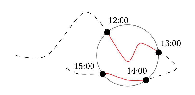
The select operator works a little different when a temporal attribute is involved in the predicate (i.e., an expression with Boolean return value). It does not tell if, but when a stream element fulfills the predictate. It does this by reducing the prediction time interval(s) to the intervals in which the predicate return true. If the prediction times are empty, i.e., if the predictate is not true at any point in time in the incoming prediction time interval(s), the stream element is removed completely.
But why are there multiple prediction time intervals, i.e., a list of time intervals, in the metadata of a steam element? That is because the predicate can be for some intervals true and for some false. The select needs to remove the intervals in which the result is false. Hence, it needs to create multiple non-intersecting time intervals. An example can be seen in the following figure. If the predicate is is_inside(tpoint, region), the result are two time intervals: [[12:00,13:00),[14:00,15:00)].
Having a list is a design decision. An alternative would have been, that the select could create multiple stream elements. Nevertheless, a select is considered to reduce the stream elements, not increasing their number. Hence, this solution was choosen.
The trimTemporal function
If the temporal attribute(s) on which an expression in a select operator is evaluated is a GenericTemporalType, i.e., a map from points in times to values, the trimTemporal function is useful. The select operator only changes the PredictionTimes metadata. For example, it limits the metdata from containins 100 points in time to 1 point in time. In that case, a GenericTemporalType temporal attribute contains 100 values but only needs to hold 1 value. The trimTemporal function removes all values instead of the ones which are within the metadata. This can reduce the memory consumption and makes the temporal attributes simpler to read in the output. On an algebraic level, this function changes nothing, as future functions will only use those values which are valid in the predictionTimes interval, anyway.
testSelect = SELECT({
	predicate = 'tdistance > 15000'
},calcDistance)

testTrim = MAP({
	expressions = ['TrimTemporal(tdistance, PredictionTimes)']
},testSelect)
Join
When applying a join operator on two streams with PredictionTimes metadata, the operator intersects the PredictionTimes to create the result element. The predicate is handled equally as in the select operator.
tempJoinTest = JOIN({
	predicate = 'other_temp_x + center_temp_x > 19'
},renameCenter,renameOther)
Aggregation
If the aggregation operator is used with a temporal attribute, the TTemporalAggregationAORule makes a few changes, but uses the same operator implementation:
- A union merge function for the PredictionTimes is applied. This leads to a result that ignores if some elements that participate in an aggregation are not valid in the prediction time dimension at some points in time, which is probably what the user wants. An intersection could be useful in some situations, but is not the default option in the implementation.
- Most aggregation functions are incremental functions. Currently, only those are supported to work with temporal attributes. They are translated to a
TemporalIncrementalAggregationFunction, which creates a temporal output for the function.
Examples
In the following, a few examples that use the temporal feature are presented.
Energy Consumption
Imagine you have a few smart meters that send you the current total energy value in an interval of 15 minutes. You need to know the consumption in-between these measurements or you want to know which households are consuming a high amount of energy right now. The following query does that for you. It takes the energy consumption and converts it into temporal attributes. Then the prediction time is set to the next 15 minutes. The derivative function can be used to get the wh per minute. Finally, the select operator selects the points in time where the consumption is "high".
#PARSER PQL
#DOREWRITE false

#DEFINE PATH_LOCAL '/media/mydata/dev/odysseus_workspace/phd-workspace/Moving Object/Evaluation/scenarios/energy/energy_data.csv'
#ADDQUERY


input = ACCESS({
            source='households',
            wrapper='GenericPull',
            schema=[
              ['id','Integer'],
              ['wh','Integer'],
              ['BaseDateTime','StartTimeStamp']
            ],
            inputschema=['Integer','Integer','Integer'],
            transport='File',
            protocol='csv',
            datahandler='Tuple',
            metaattribute = ['TimeInterval',  'PredictionTimes'],
            options=[
              ['filename', ${PATH_LOCAL}],
              ['Delimiter',','],
              ['TextDelimiter','"'],
              ['delay','1000'],
              ['readfirstline','false'],
              ['BaseTimeUnit','MINUTES']
            ]
          }
        )

/// Only use the last two measured values
time = TIMEWINDOW({
            size = [20, 'minutes']
          },
          input
        )

/// Convert the wh-attribute to a temporal double
temporalize = AGGREGATION({
                  aggregations = [
                    ['function' = 'ToTemporalDouble', 'input_attributes' = 'wh', 'output_attributes' = 'temp_wh']
                  ],
                  group_by = ['id'],
                  eval_at_outdating = false
                },
                time
              )

predTime = PREDICTIONTIME({
                addtostartvalue = [0, 'MINUTES'],
                addtoendvalue = [15, 'MINUTEs']
              },
              temporalize
            )


/// Energy consumption per household per minute in the next 15 minutes
derivative = MAP({
                  expressions = [
                    ['derivative(temp_wh, PredictionTimes)','whPerMinute'],
                    ['id','id']
                  ]
                },
                predTime
              )

/// Energy consumption per household per minute in the next 15 minutes
watts = MAP({
                  expressions = [
                    ['whPerMinute * 60','watt'],
                    ['id','id']
                  ]
                },
                derivative
              )

/// Filter out elements with a low energy consumption
highConsumption = SELECT({
                      predicate = 'watt > 300'
                    },
                    watts
                  )
And here's an example file with energy consumption data:
id,wh,time
1,0,0
2,0,3
3,0,6
1,115,15
2,50,18
3,250,21
1,200,30
2,60,33
3,500,36
1,210,45
2,100,48
3,600,51