One important operation in streaming and CEP applications is the aggregation. We will give an example on how Odysseus computes aggregations. A problem for aggregations in combination with sliding windows is how to handle events which leave a window (they become invalid). A simple approach is to keep every event and calculate the aggregation on evaluation time. Here, the event that get invalid can be simply removed. But this causes a large memory overhead. Odysseus adapts the concept of online aggregations. In this concept, only the minimal needed information is kept to calculate an aggregation over a window by utilizing so called partial aggregates. A very intuitive example is the calculation of an average: The partial aggregate needs to keep a running sum and the count of events aggregated so far. This can be used to calculate the concrete result anytime by the division of sum and count.
But with this partial aggregates, it is not possible to remove the values of the first event without knowing its content. In Odysseus we adapted the approach of Partial aggregates. Partial aggregates are built only from events that overlap in their time interval. For this, new events must be combined with different existing partial aggregates. The following figure illustrates an example.
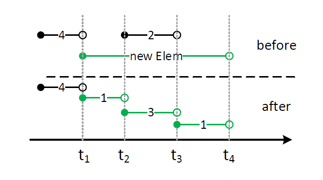
To make the gure more readable, this example shows a count aggregation. The AGGREGATE operator keeps a state of all current partial aggregates.
In this example there are two partial aggregates with the count 4 and the count 2 in the upper part of the figure. If a new event arrives at the system (here with the validity from t1 to t4), the new event has to be compared with all contained events. The lower area shows the result of the processing. The event with count the 4 is not treated as it does no overlap with the new event. From t1 to t2 a new event with the count 1 is inserted, analogous from t3 to t4. Within the range from t2 to t3, an overlapping occurs. The new partial aggregate is derived from the old one with the new event, leading to a new partial aggregate with the count 3.
The final question is: When can any of the contained event be evaluated and sent to the next operator? This depends on how time progress is determined. When the stream is ordered by start time stamp, the partial aggregate with the count 4 will not be used anymore because every following event must have a time stamp higher that t1 and the partial aggregate can be removed from the state and sent to the next operator.
A special case is the treatment of groups, e.g., if not all elements should be counted, but the elements with a special attribute value (e.g. the count of bids for an auction). In this case, the AGGREGATE operator keeps an own state for each group and provides special handling for out of order events. is used to aggregate and group the input stream.
Parameter
group_by:An optional list of attributes over which the grouping should occur.aggregations:A list if elements where each element contains up to four string:- The name of the aggregate function, e.g. MAX
- The input attribute over which the aggregation should be done. This can be a single value like
'price'or for some aggregate function a list['price','id']or'*'for all Attributes. The latter one can be used for aggregations where so single attribute is relevant, e.g. with COUNT - The name of the output attribute for this aggregation
- The optional type of the output. If not given, DOUBLE will be used.
dumpAtValueCount:This parameter is used in the interval approach. Here a result is generated, each time an aggregation cannot be changed anymore. This leads to fewer results with a larger validity. With this parameter the production rate can be raised. A value of 1 means, that for every new element the aggregation operator receives new output elements are generated. This leads to more results with a shorter validity.outputPA: This parameter allow to dump partial aggregates instead of evaluted values. The partial aggregates can be send to other aggregation operators and do a final aggregation (e.g. in case of distribution). The input schema of an aggregate operator that read partial aggregates must state a datatype that is a partial aggregated (see example below). Remark: Aggregate has one input and requires ordered input. To combine different parital aggregations e.g. a union operator is needed to reorder the input elements.drainAtDone: Boolean, default true: If done is called, all not already written elements will be written.drainAtClose: Boolean, default false: If close is called, all not already written elements will be written.FastGrouping: Use hash code instead of compare to create group. Potentially unsafe!
New: In the standard case the AGGREGATE operator creates outputs with start and end timestamp. This could lead to higher latency because the operator has to wait for the next element to set the end time stamp. With
latencyOptimized= true
the operator creates for every new incomming element a new output and sets only the start time stamp for the output. If the input contains equals start time stamps, there will be an output for every incomming element, too. See example below.
Aggregation Functions
The set of aggregate functions is extensible. The following list is in the core Odysseus:
MAX: The maximum elementMIN: The minimum elementAVG: The average elementSUM: The sum of all elementsCOUNT: The number of elementsMEDIAN: The median elementSTDDEV: The standard deviation- VAR: The variance
- CORR: The correlation between two attributes
- COV: The covariance between two attributes
Some nonstandard aggregations: These should only be used, if you a familiar with them:
FIRST: The first elementLAST: The last elementNTH: The nth elementRATE: The number of elements per time unitNEST: Nest the attribute values in a list- DISTINCTNEST: Nest only distinct attribute values in a list
COMPLETENESS: Ratio of NULL-value elements to number of elements
Example:
PQL
| Code Block | ||||||||||
|---|---|---|---|---|---|---|---|---|---|---|
| ||||||||||
output = AGGREGATE({
                    group_by = ['bidder'],
                    aggregations=[ ['MAX', 'price', 'max_price', 'double'] ]
                   }, input)

// Parital Aggregate example
pa = AGGREGATE({
          name='PRE_AGG',
          aggregations=[
            ['count', 'id', 'count', 'PartialAggregate'],
            ['sum', 'id', 'avgsum', 'PartialAggregate'],
            ['min', 'id', 'min', 'PartialAggregate'],
            ['max', 'id', 'max', 'PartialAggregate']
          ],
          outputpa='true'
        },
        nexmark:person
      )

out = AGGREGATE({
          name='AGG',
          aggregations=[
            ['count', 'count', 'count', 'Integer'],
            ['sum', 'avgsum', 'sum', 'Double'],
            ['avg', 'avgsum', 'avg', 'Double'],
            ['min', 'min', 'min', 'Integer'],
            ['max', 'max', 'max', 'Integer']
          ]
        },
        pa
      )

/// Example for aggregations on multiple attributes
out = AGGREGATE({
          aggregations=[
            ['corr', ['x', 'y'], 'correlation', 'Double'],
            ['cov', ['x', 'y'], 'covariance', 'Double']
          ]
        },
        input
) |
CQL
| Code Block | ||||||||||
|---|---|---|---|---|---|---|---|---|---|---|
| ||||||||||
SELECT MAX(price) AS max_price FROM input GROUP BY bidder |
Latency Optimized
The latency optimized version of the operator does not create time intervals for the output but sets only the start time stamp. This has the advantage, that for every state change a new element is created.
Here is an example to see the difference.
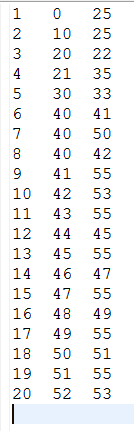
Suppose an input as following:
For the non latency optimized (default) case:
| Code Block |
|---|
#PARSER PQL
#IFSRCNDEF overlapping
#RUNQUERY
overlapping := ACCESS({
                    source='overlapping ',
                    wrapper='GenericPull',
                    transport='file',
                    protocol='simplecsv',
                    datahandler='tuple',
                    schema=[
                      ['a1', 'integer'],
                      ['start', 'startTIMESTAMP'],
                      ['end', 'endTIMESTAMP']
                    ],
                    options=[
                      ['filename', '${PROJECTPATH}/overlappingInput.csv'],
                      ['delimiter', '\t']
                    ]
                  }
                )
#endif
#RUNQUERY
out = AGGREGATE({
          aggregations = [['COUNT', '*', 'counter']]
        },
        overlapping
) |
the output will be as follows:
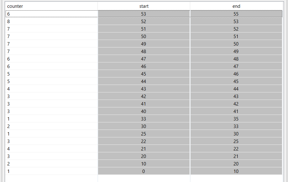
Here you can see start and end time stamps in the output.
For the latency optimized case:
| Code Block |
|---|
#PARSER PQL

#RUNQUERY
out = AGGREGATE({
          aggregations = [['COUNT', '*', 'counter']], LatencyOptmized = true
        },
        overlapping
) |
the output differs:
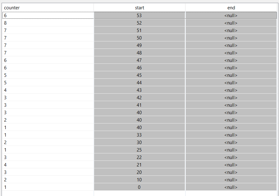
The most obvious thing is: There are no end time stamps.
But there is one more thing different. In the standard case above there is for each start time stamp only one value (see 40), and here for each incoming tuple a value.